Accelerating PyTorch: Custom CUDA Extensions for Unparalleled Performance

Introduction

Although creating custom CUDA extensions to try to improve the performance of PyTorch may sound daunting, it is simpler than you may think. I have a lot of experience in PyTorch coming from an ML background but only have recently picked up on CUDA programming from taking a Parallel Programming Course. I hope this blog post shows how even a relative beginner at CUDA can come up with a specific application, write a CUDA kernel to speed it up, wrap that CUDA kernel so that it can be executed in Python and use it in downstream tasks.

Inspiration

The algorithm I chose to focus on is the Cross-Entropy Method Algorithm.
The inspiration from this comes from the algorithm that almost perfectly plays Tetris.
If you look at the best Tetris-playing bot, you will see that the Cross-Entropy Method is the leader even compared to neural network-based approaches that exist today.
Here is the algorithm in my own words:

Compute all possible next moves(Where/What block you will place)
For each next state of the game, compute features for that state.
Weight each feature by a weight $w_i$ and sum them up to get a value for the possible next states.
Choose the action that takes you to the state with the largest value.
Repeat

Here are the commonly used features in the algorithm:

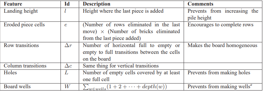
If you look at step 3, we need to figure out good weights for each of these features to determine how good a state is.

How do we do that?

That’s where the Cross Entropy Method comes into play.
We first start with a vector of random weights $\mu$ and $\sigma$ vector of the standard deviation of each of those weights(ex: all 1 at the beginning)
Then we apply the CEM algorithm as shown below:
Here is an Overview of the algorithm:

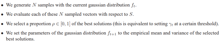
Here is a visual representation of that same algorithm:

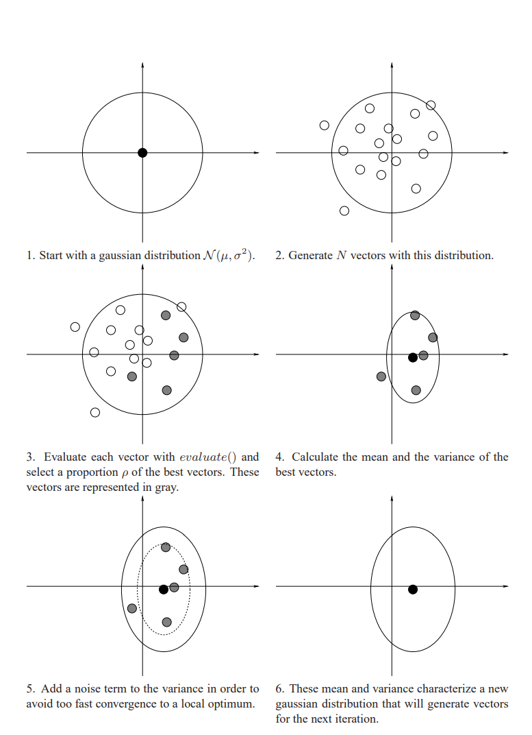
This is very similar to evolutionary algorithms, and by using CEM for many iterations, slowly the weights you choose will become better and better.

The CEM algorithm has 4 main steps, but I decided to try and speed up the first step: Generate N random Vectors from a Normal Distribution
This step is the most general and is used everywhere in scientific computing and is a very general operation.

Algorithm

If we focus on how to sample from a Normal Distribution, we can use the following formulation.

$X \sim N(\mu, \sigma^2)$

$X = \mu + Z\sigma$

$Z \sim N(0,1)$

We can extend this to multi-dimension vectors as follows: Lets say our $\mu$ and $\sigma$ are d dimensional vectors and we are trying to sample N random vectors:

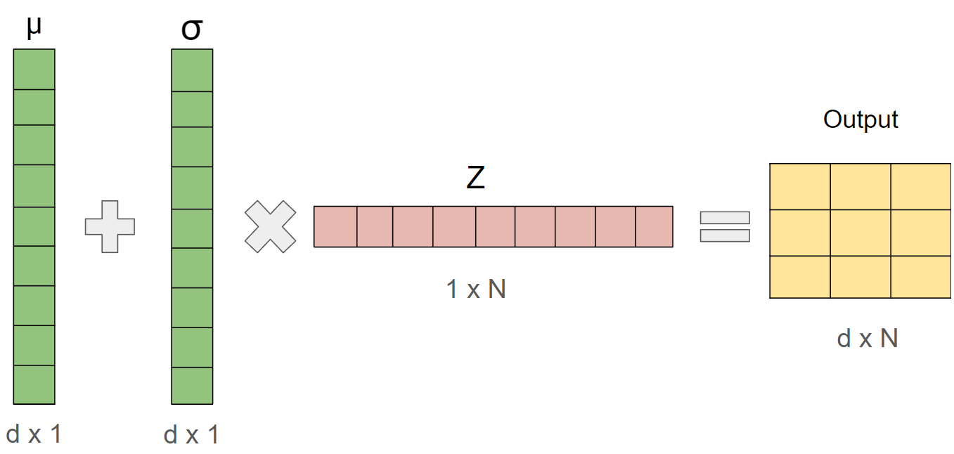
With the Broadcasting of these tensors, we end up with a tensor of shape (d x N) which represents our N randomly sampled vectors of dimension d which is our desired output.

Pytorch Implementation

Implementing this in Pytorch is very simple. We can implement it just like the equation above.

import torch
num_samples = 1024
vector_dim = 2500
mu = torch.randn((vector_dim,1),device="cuda")
sigma = torch.randn((vector_dim,1),device="cuda")
output = mu + sigma * torch.randn((1,num_samples),device="cuda")

How to Develop CUDA custom C++ extensions for PyTorch

Before we get into how to develop the CUDA equivalent of this operation, I want to go over how to create CUDA C++ extensions for Pytorch so that you can run your efficient CUDA code in PyTorch.

The steps are roughly as follows:

Write a normal cuda kernel with the types you want in a .cu file using the support and IDE gives you(Linting etc.)
Write a main function in the file to test that gpu code to see if it does what is expected. For example, create a c++ array with the same values as in your pytorch tensor, run the code and make sure both output are close to the same values.
Add the small amount of PyTorch overhead needed in your cpp file

CUDA Implementation

The way I went about parallelizing this code is to have each block on the GPU deal with one of the d rows of the output(So deal with one of the dimensions of the vector)

Each thread in the block deals with computing one of the N samples This means the launch parameters for our kernel are: Threads Per Block(TPB) = Number of samples N, Number of Blocks = Vector Dimension d

The math each thread computes is identical to the Pytorch version.

Since in most CUDA GPUs, the max threads per block is 1024, the maximum number of samples we can have is 1024 with this strategy(This is a reasonable number in practice).

Here is the .cu code that defines the cuda kernel that computes the output given the input $\mu$ , $\sigma$ and $Z$ vectors:

#include <cuda_runtime_api.h>
#include <cuda.h>
#include <curand.h>
#include <c10/cuda/CUDAException.h>
/*
Lets try to create a fast GPU normal dist sampling algorithm:
It will require this kernels:
Sample: Input = mu,sigma 1d-vectors, N where N is number of vectors to sample. Output: d*N matrix of vectors
We can parallelize over each element in the mu,sigma vector and then have each thread write N numbers
*/

// Threads parallelize over N, blocks parallelize over d
__global__ void sample(float *d_mu, float *d_sigma, float *d_rand, float *d_output, int d, int N)
{
    int dimension_id = blockIdx.x;
    int sample_id = threadIdx.x;

    d_output[dimension_id * N + sample_id] = d_mu[dimension_id] + d_sigma[dimension_id] * d_rand[sample_id];
}

void sample_gpu(int d, int num_samples, float *d_mu, float *d_sigma, float *d_output, float *d_rand)
{
    sample<<<d, num_samples>>>(d_mu, d_sigma, d_rand, d_output, d, num_samples);
    C10_CUDA_KERNEL_LAUNCH_CHECK();
}

Here is the cpp code that acts as a wrapper for the cuda kernel to work with PyTorch tensors and to use it as a module in Python:

#include <torch/extension.h>
#include "ATen/ATen.h"
#define CHECK_CUDA(x) TORCH_CHECK(x.device().is_cuda(), #x " must be a CUDA tensor")
#define CHECK_CONTIGUOUS(x) TORCH_CHECK(x.is_contiguous(), #x " must be contiguous")
#define CHECK_INPUT(x) \
    CHECK_CUDA(x);     \
    CHECK_CONTIGUOUS(x)

void sample_gpu(int d, int num_samples, float *d_mu, float *d_sigma, float *d_output, float *d_rand);

torch::Tensor sample(torch::Tensor mu, torch::Tensor sigma, int num_samples)
{
    CHECK_INPUT(mu);
    CHECK_INPUT(sigma);
    int d = mu.size(0);
    auto output = torch::zeros({d, num_samples}, mu.options());
    auto rand = torch::randn({num_samples}, mu.options());
    sample_gpu(d, num_samples, mu.data_ptr<float>(), sigma.data_ptr<float>(), output.data_ptr<float>(), rand.data_ptr<float>());
    return output;
}

PYBIND11_MODULE(TORCH_EXTENSION_NAME, m)
{
    m.def("sample", &sample, "gpu normal dist sampling");
}

We can see that the cpp file is very simple and essentially it just calls the function we defined in the .cu file. Additionally, it creates the output tensor to store the results of the operation and the input random vector. It also does a check to make sure that the tensor is on the GPU and that it is contiguous in memory.

Once you write your sample.cu and sample.cpp files as shown above, loading them in Python is very easy:

from torch.utils.cpp_extension import load
sample_lib = load(name="sample", sources=["sample.cu", f"sample.cpp"],
                    verbose=True, extra_cuda_cflags=["-res-usage", "--use_fast_math", "-O3", "-Xptxas -O3", "--extra-device-vectorization"])
//Example of how to call function
output = sample_lib.sample(mu,sigma,num_samples)

Benchmarks

The GPU that I used to benchmark this code was the GPU in my local laptop: RTX 3070
Although this is quite an old GPU model, it can still show how efficient our kernel is on the GPU.
Since the kernel I defined could have a max number_of_samples = 1024(sufficient in practice) I fixed the number_of_samples to be 1024 and benchmarked the PyTorch and CUDA kernels while varying the dimension d of the vector.

To properly benchmark gpu kernels, using cuda events is the best way to go about it.
Clearing the cache is important when running a kernel multiple times since the algorithm will likely run faster when memory is loaded into the cache.
Starting to time kernels after a few warmup calls can also help, since GPUs can be slow on the first few kernel calls.
Here is an example of the Python timing code that uses Cuda events, incorporates warmup, and clears the cache every time:

times = []
torch.cuda.empty_cache()
for i in range(1000):
    start.record()
    samples = sample_lib.sample(mu,sigma,num_samples)
    end.record()
    torch.cuda.synchronize()
    torch.cuda.empty_cache()
    if i > warmup_steps:
        times.append(start.elapsed_time(end) / 1000)
my_time = torch.mean(torch.tensor(times))
print(f'My Kernel Avg Time Taken(s): {my_time}')

torch.compile is a Pytorch 2.0 feature that helps compile a torch function and possibly optimize it by fusing kernels and other optimizations. Using it is as simple as this:

def sample_torch(num_samples,mu,sigma):
    return mu + sigma * torch.randn((1,num_samples),device="cuda")
compiled_sample_torch = torch.compile(sample_torch)

I decided to include the compiled code in the benchmark as well.
I ran each kernel 1000 times and average the time taken for the kernel for different vector dimensions d
Here is a plot of those runtimes:

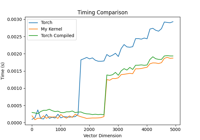
Since the compiled function is faster than the PyTorch kernel on average, I decided to not include the normal PyTorch kernel in the next visualization.
The Speedup of our kernel = (Compiled Torch Time/ My Kernel Time)
I decided to plot the speedup of my kernel compared to the Compiled PyTorch kernel as well for different vector dimensions d:

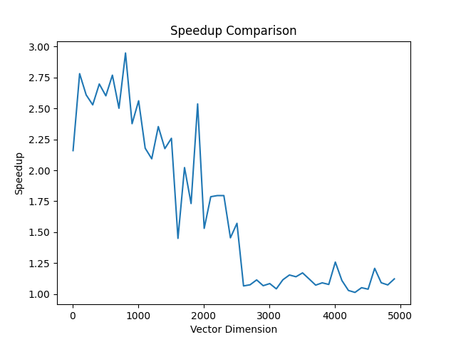
We can see that on average, across all vector sizes form (10-5000), on average the speedup of our kernel is: 1.66 x
That’s close to a 66% increase in performance on average!!!!

Conclusion

We can see that the compiled torch code is much faster at larger vector sizes than the raw PyTorch code.
The speedup we see that my kernel achieves compared to the raw PyTorch kernel could be due to “Kernel Fusion” where our method combines all the operations into one kernel as opposed to calling a multiply kernel and an add kernel.
What is cool is that our method is a good amount faster than torch.compile on most vector sizes and much faster(close to 2.5x on vector sizes ranging from (10-1000)).
Pytorch is quite optimized and torch.compile usually creates very efficient code so being able to speed up performance on all vector sizes is great and could be very useful in the many algorithms that use it a lot like CEM.

Overall tackling this problem was a great way for me to learn more about how to create CUDA extensions for PyTorch and helped me get exposure to how to speed up code for a certain task.

I have uploaded all the code to Github if you would like to run the benchmarks yourself on your own computer: Github

Many more optimizations could be done to this code.
The next steps, if you wanted to squeeze out more performance from this code, would be to use a profiler like NCU to determine the bottlenecks in the code and use optimizations like using shared memory and techniques like thread-coarsening or more advanced techniques.

I would appreciate any feedback in the comments on how I could make this algorithm even faster on what the runtimes look like on much more modern GPUs and if the trends still hold.

Thanks For Reading :)

Blog Archive

Archive of all previous blog posts

Blog Archive

Archive of all previous blog posts